Diodes are electronic devices that conduct in one direction. Ideally, they have to block the conduction of current in the reverse direction, but in reality, there is always a small leakage current present.
Due to the presence of impurities in the diode, it gets hot when a large amount of current is passed through.
There are diodes for various applications which focus on a special property of the diode.
For example:
Zener Diode – Works in reverse bias condition. Provide excellent voltage regulation.
Schottky Diode – Has low forward voltage drop and high switching speed. Suitable for high-frequency applications and power supply circuits.
Silicon Controlled Rectifier (SCR) – Can handle high current and voltage levels. Used for power switching and motor control applications.
Light Emitting Diode (LED) – Emits light when forward biased. Used for lighting and display applications.
Tunnel Diode – Exhibits negative resistance. Used in microwave oscillators, amplifiers, and detectors.
Avalanche Diode – Can withstand high reverse voltage and exhibits avalanche breakdown. Used for overvoltage protection and voltage regulation.
Photodiode – Generates a current when exposed to light. Used in optical communication and sensing applications.
These are just a few examples, and there are many more types of diodes available for various applications.
The following properties should be looked at in a datasheet. There may be additional details but these are the minimum.
VFis the voltage drop across the diode when it is conducting current in the forward direction. For example, a silicon diode may have a VF of around 0.7V.
IFis the maximum current that the diode can handle without being damaged. For example, a diode rated for 1A can handle a maximum current of 1A flowing through it.
VRis the maximum reverse voltage that the diode can withstand before breakdown. For example, a diode with a VR of 100V can withstand a reverse voltage of up to 100V before it starts conducting in the reverse direction.
PDis the maximum power that the diode can safely dissipate without getting damaged. For example, a diode with a PD of 500mW can safely dissipate up to 500mW of power without getting damaged.
Tjis the maximum temperature that the junction of the diode can reach without getting damaged. For example, a diode with a Tj of 150°C can safely operate at a maximum temperature of 150°C.
trris the time taken by the diode to switch from forward conduction to reverse blocking mode. For example, a diode with a trr of 50ns will take 50ns to switch from forward conduction to reverse blocking mode.
The package type and dimensions specify the physical size and shape of the diode and are usually given in the mechanical drawing section of the datasheet. For example, a diode may be packaged in a through-hole or surface-mount package with specific dimensions.
Electronic Diodes and Their Part Numbers
Rectifier Diodes
Small Signal Diode: 1N4148, 1N914
Schottky Diode: BAT54, BAT85
Silicon Controlled Rectifier: TYN616, C106D
PIN Diode: HP5082-2810, HSMP-386L
Zener Diodes
Zener Diode: 1N4728A, 1N5349B
LED and Laser Diodes
Light Emitting Diode (LED): 5mm Red LED, 3mm Green LED
Laser Diode: 650nm Red Laser, 405nm Blue Laser
Special Function Diodes
Tunnel Diode: 1N3716, NTT406AB
Varactor Diode: BB112, BB204
Transient Voltage Suppression Diode: P6KE36A, 1.5KE200A
Avalanche Diode: BZX84C5V6, P6KE100CA
Photodiodes
PIN Photodiodes: BPW34, SFH205F
Avalanche Photodiodes: S8664, C30932EH
Schottky Photodiodes: 1N5711, HSMS-2855-BLKG
MSM Photodiodes: YT201M, YT202M
InGaAs Photodiodes: G9933, G8941
Power Diodes
General Purpose Power Diodes: 1N4007, 1N5399
Fast Recovery Power Diodes: UF4007, FR107
Schottky Barrier Diodes: SB560, SB5100
Ultrafast Recovery Power Diodes: UF5404, UF5408
Super Barrier Diodes: SB540, SB570
Avalanche Diodes: MUR1100E, 1N4937GP
TVS Diodes (Transient Voltage Suppressor): P6KE15CA, 1.5KE400A
In Tkinter, the sticky option is used to specify how a widget should expand to fill the space allotted to it within its container widget.
The sticky option is used when placing a widget using the grid geometry manager. When a widget is placed in a cell of the grid, it can be set to “stick” to one or more sides of the cell. The sticky option takes one or more of the following values:
N: stick to the top edge of the cell
S: stick to the bottom edge of the cell
E: stick to the right edge of the cell
W: stick to the left edge of the cell
NW: stick to the top-left corner of the cell
NE: stick to the top-right corner of the cell
SW: stick to the bottom-left corner of the cell
SE: stick to the bottom-right corner of the cell
For example, if you want a widget to fill the entire width of a cell and stick to the top edge of the cell, you can use:
This will place the widget in the first row, first column of the grid, and span two columns. The sticky option is set to 'W' + 'E' + 'N', which means the widget will stick to the left, right, and top edges of the cell, but not the bottom edge. As a result, the widget will expand horizontally to fill the width of the cell, but not vertically.
Example
import tkinter as tk

root = tk.Tk()

# Create a label widget and place it in the first row, first column of the grid
label = tk.Label(root, text="Hello, world!")
label.grid(row=0, column=0)

# Create a button widget and place it in the second row, first column of the grid
button = tk.Button(root, text="Click me!")
button.grid(row=1, column=0)

# Create an entry widget and place it in the second row, second column of the grid
entry = tk.Entry(root)
entry.grid(row=1, column=1, sticky='W')

# Create a text widget and place it in the third row, first column of the grid
text = tk.Text(root)
text.grid(row=2, column=0, columnspan=2, sticky='W'+'E'+'N'+'S')

branding_label = tk.Label(root, text="Powered by exasub.com")
branding_label.grid(row=3, column=0, columnspan=2, padx=10, pady=10, sticky='E')

root.mainloop()
In this example, we create a label widget, a button widget, an entry widget, and a text widget, and place them in a grid using the grid geometry manager.
The label widget is placed in the first row, first column of the grid, with no sticky option specified, so it will not expand to fill the cell.
The button widget is placed in the second row, first column of the grid, with no sticky option specified, so it will not expand to fill the cell.
The entry widget is placed in the second row, second column of the grid, with the sticky option set to ‘W’, so it will stick to the left edge of the cell and not expand to fill the cell.
The text widget is placed in the third row, first column of the grid, with the sticky option set to ‘W’+’E’+’N’+’S’, so it will stick to all four edges of the cell and expand to fill the entire cell.
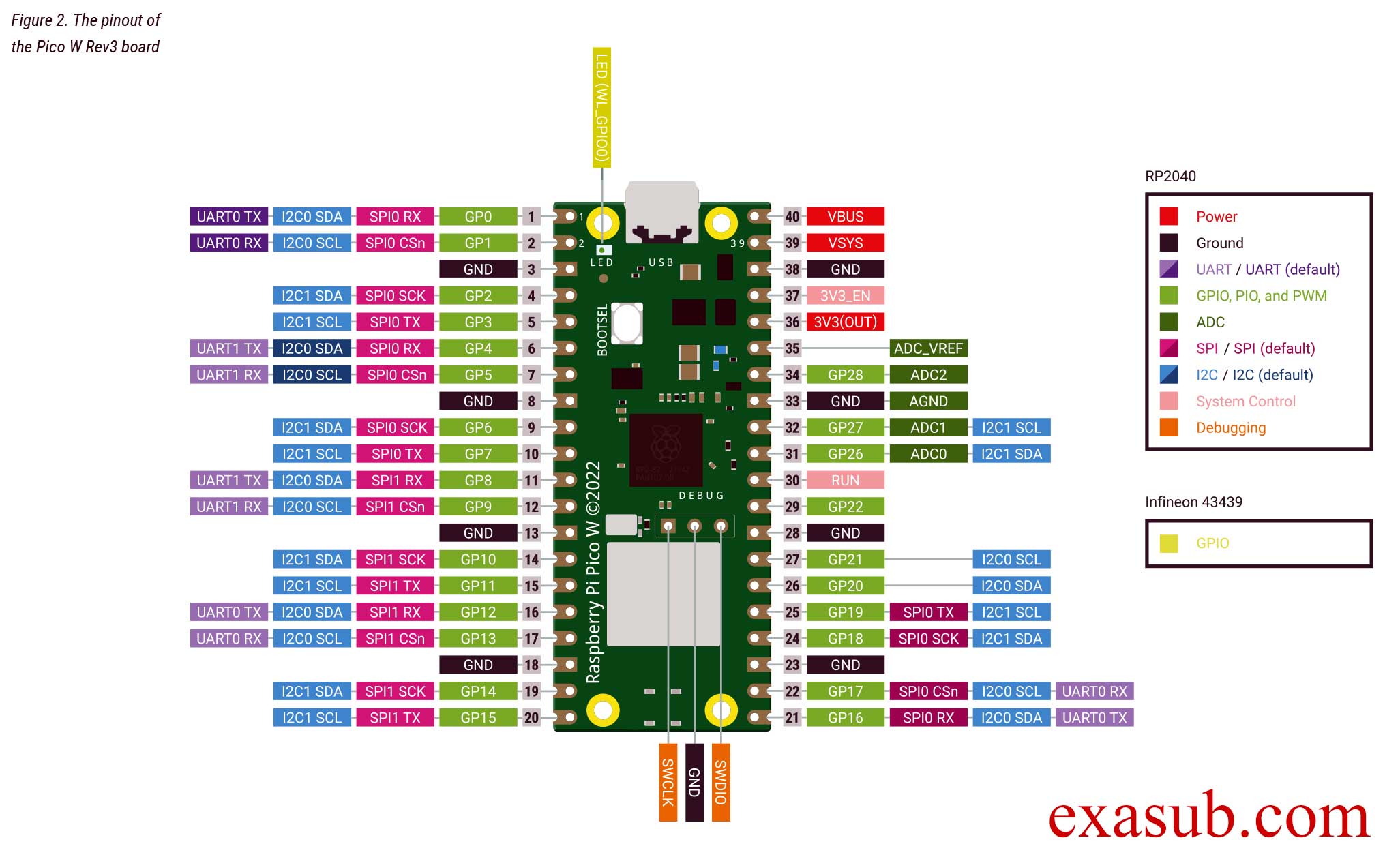
The raspberry pi pico w has a LED on it. This LED is not connected to the GPIO pins of RP2040 microcontroller directly.
As you can see in the image of the pinout taken from the official datasheet. The onboard LED is connected to a pin ‘WL_GPIO0’. WL_GPIO0 is an internal pin.
There are different ways to program the pico W. The easiest method is to install thonny IDE. And install micropython on the pico w.
After you have installed thonny. Now connect you raspberry pi pico w board to the computer USB port while holding the onboard BOOTSEL button. Then follow the steps shown in the following images.
Step 1Step 2Step 3step 4. Click Install after this.
After you have done the above steps. You now have to install a MicroPython library.
picozero is a MicroPython library which has functions for Wifi and other RP2040 chip.
To complete the projects in this path, you need to install the picozero library as a Thonny package.
In Thonny, choose Tools > Manage packages.
Code
import machine
import time

# create a Pin object to control the LED on pin 'WL_GPIO0'
led_pin = machine.Pin('WL_GPIO0', machine.Pin.OUT)

# enter an infinite loop
while True:
    # set the LED pin to a high (on) state
    led_pin.value(1)
    # pause the program for one second
    time.sleep(1)
    # set the LED pin to a low (off) state
    led_pin.value(0)
    # pause the program for one second
    time.sleep(1)
In this program, we first import the machine module and the time module. The machine module provides access to hardware-level features on the Raspberry Pi Pico, while the time module provides functions for time-related operations.
Next, we create a Pin object called led_pin to control the LED connected to the pin labeled ‘WL_GPIO0’. The machine.Pin() function is used to create the led_pin object, with the first argument specifying the pin label and the second argument specifying that the pin is an output pin, i.e. we can set its state to high or low.
Then, we enter an infinite loop using the while True: statement. Within the loop, we use the value() method of the led_pin object to set the state of the LED pin to high (on) or low (off), with a one second delay between each state change using the time.sleep() function.
Comments are added to explain each line of code and make it easier to understand the purpose and function of the program.
The Raspberry Pi 3B+ is powered by a Broadcom BCM2837B0 chipset, which includes a 1.4 GHz 64-bit quad-core ARM Cortex-A53 CPU.
The BCM2837B0 also includes a VideoCore IV GPU, which is capable of hardware-accelerated video decoding and encoding, 3D graphics rendering, and image processing.
The Raspberry Pi 3B+ comes with 1 GB of LPDDR2 SDRAM memory, which is shared between the CPU and GPU.
The LPDDR2 SDRAM on the Raspberry Pi 3B+ runs at 900 MHz, providing a maximum memory bandwidth of 7.2 GB/s.
The Raspberry Pi 3B+ also supports virtual memory, which allows it to use a portion of its SD card storage as swap space to increase the available memory.
The BCM2837B0 chipset includes a level 2 (L2) cache of 512 KB, which is shared between all four CPU cores.
The L2 cache on the Raspberry Pi 3B+ runs at the same speed as the CPU cores (1.4 GHz), providing fast access to frequently used data and instructions.
The BCM2837B0 chipset also includes a hardware random number generator, which can be used for cryptographic applications that require secure and unpredictable random numbers.
Connectivity
Ethernet: Gigabit Ethernet over USB 2.0 (maximum throughput 300 Mbps)
Wireless: 2.4GHz and 5GHz IEEE 802.11.b/g/n/ac wireless LAN
Bluetooth: Bluetooth 4.2, Bluetooth Low Energy (BLE)
Storage
microSD card slot for loading operating system and data storage
The Raspberry Pi 3B+ has a microSD card slot that supports the use of microSD, microSDHC, and microSDXC cards.
The microSD card slot on the Raspberry Pi 3B+ supports UHS-I bus speeds, which can provide faster data transfer rates than standard SD cards.
The Raspberry Pi 3B+ also supports booting from USB mass storage devices, such as USB flash drives or external hard drives.
The Raspberry Pi 3B+ supports the use of file systems such as ext4, NTFS, and FAT32 on external storage devices.
The maximum recommended microSD card size for the Raspberry Pi 3B+ is 32 GB, although larger cards can be used with some limitations.
Multimedia
Video: H.264 (up to 1080p60), MPEG-4 (up to 1080p30), H.263 (up to 1080p30)
Audio: Stereo audio via 3.5mm jack, or HDMI
GPIO
40-pin GPIO header with support for SPI, I2C, and UART protocols
40 GPIO pins are available in two rows of 20 pins each on the GPIO header.
The GPIO pins on the Raspberry Pi 3B+ operate at 3.3V logic levels and are not 5V tolerant. Connecting 5V devices directly to the GPIO pins can damage the Raspberry Pi.
The GPIO pins can source or sink up to 16 mA of current.
The GPIO pins can be configured as inputs or outputs, and can also be used for hardware PWM (Pulse Width Modulation) and hardware SPI (Serial Peripheral Interface) communication.
The GPIO pins are grouped into several GPIO banks, each with its own set of features and capabilities. These banks include the General Purpose Input/Output (GPIO) bank, the Serial Peripheral Interface (SPI) bank, the Inter-Integrated Circuit (I2C) bank, and the Universal Asynchronous Receiver-Transmitter (UART) bank.
The GPIO pins on the Raspberry Pi 3B+ can be accessed using a variety of programming languages and libraries, including Python, C, C++, and Node.js. The RPi.GPIO library, which is included with the Raspbian operating system, provides a simple and easy-to-use interface for controlling the GPIO pins using Python. Additionally, it is possible to access the GPIO pins using bare metal programming, which involves programming the Raspberry Pi directly without using an operating system. This method provides more control over the hardware and can be useful in applications where performance and real-time control are critical.
Bare metal programming is the practice of programming a computer or microcontroller without using an operating system or any other software layer between the hardware and the code. It involves writing code that directly interacts with the hardware, using low-level programming languages such as Assembly or C. This allows for greater control over the hardware, as you have direct access to the processor, memory, and other resources.
In the case of Raspberry Pi, bare metal programming involves writing code directly to the hardware, using low-level programming languages such as Assembly or C.
Advantages
Disadvantages
Provides direct access to the hardware, enabling greater control over system resources
Requires advanced knowledge of low-level programming languages such as Assembly or C
Avoids the overhead and complexity of operating systems and middleware
Requires more effort and time to develop and maintain code compared to high-level programming languages or using an operating system
Enables faster and more efficient code execution
Lack of abstraction and protection from hardware errors can lead to more complex and error-prone code
Ideal for applications with strict timing requirements or low-latency communication with hardware peripherals
Difficult to integrate with higher-level software stacks or libraries
To get started with bare metal programming on Raspberry Pi 3B+, you’ll need the following tools:
Raspberry Pi 3B+: This is the main hardware component you’ll need to get started with bare metal programming on Raspberry Pi.
MicroSD card: You’ll need a MicroSD card to store the operating system and your code. A capacity of 8GB or higher is recommended.
Cross-compiler: This is a toolchain that allows you to compile your code on a different platform (such as a PC) and generate code that can run on the ARM-based Raspberry Pi. You can use the GNU ARM Embedded Toolchain or other cross-compilers.
Text editor: You’ll need a text editor to write and edit your code. Some popular free options include Notepad++, Nano, and Visual Studio Code.
This code is a Resistor Color Code Calculator. A resistor is an electronic component used in circuits to control the flow of electricity. The colors of the bands on the resistor indicate the resistance value of the resistor. This code allows you to select the color of the four bands on the resistor and then calculate the resistance value of the resistor.
The code uses a graphical user interface (GUI) built using a library called tkinter. The GUI consists of labels, dropdown menus, a button, and a link. The dropdown menus allow you to select the colors of the four bands on the resistor. The button, when pressed, calculates the resistance value of the resistor and displays it on the screen. The link is a hyperlink that takes you to a website.
The code defines two dictionaries that hold the color codes and tolerance values for resistors. The calculate_resistance function uses the selected colors to calculate the resistance value of the resistor. The open_website function opens a website when the link is clicked.
A digital clock is a very common type of clock that displays the time in digits, as opposed to an analog clock that displays the time using clock hands. With Python, you can easily create a digital clock using the Tkinter GUI toolkit. In this article, we will show you how to create a digital clock using Python.
Step 1: Importing Required Libraries We need to import the following libraries to create a digital clock in Python:
from tkinter import *
import time
Here, we import the Tkinter library for creating the graphical user interface, and the time library for working with time and dates in Python.
Step 2: Creating the Digital Clock Class We will create a class called DigitalClock that contains the code for creating the digital clock.
class DigitalClock:
    def __init__(self, root):
        self.root = root
        self.root.title("Digital Clock")
        self.root.geometry("300x200")
        self.root.resizable(False, False)

        # Create a label for displaying the current time
        self.time_label = Label(root, text="", font=("Arial", 50))
        self.time_label.pack(pady=20)

        # Add your website name with a hyperlink
        self.link_label = Label(root, text="exasub.com", font=("Arial", 14), fg="blue", cursor="hand2")
        self.link_label.pack(pady=10)
        self.link_label.bind("<Button-1>", lambda event: self.open_website())

        # Update the time every second
        self.update_clock()
Here, we define the __init__ method that initializes the class with the root argument. We set the title of the window to “Digital Clock”, and set the window size to 300×200. We then create a label called time_label to display the current time with a font size of 50.
We also create another label called link_label that displays your website name with a hyperlink. When the user clicks on the link, the open_website method will be called.
Finally, we call the update_clock method to update the time every second.
Step 3: Updating the Clock We will now define the update_clock method that will update the clock every second.
def update_clock(self):
    # Get the current time and format it
    current_time = time.strftime("%H:%M:%S")
    self.time_label.config(text=current_time)

    # Schedule the next update after 1 second
    self.root.after(1000, self.update_clock)
Here, we get the current time using the strftime method of the time library, and format it in the HH:MM:SS format. We then set the text of the time_label to the current time using the config method.
We also schedule the next update after 1 second using the after method of the root window.
Step 4: Opening the Website We will define the open_website method that will open your website when the user clicks on the hyperlink.
Here is the complete code for creating a digital clock using Python:
from tkinter import *
import time
class DigitalClock:
def __init__(self, root):
self.root = root
self.root.title("Digital Clock")
self.root.geometry("300x200")
self.root.resizable(False, False)
# Create a label for displaying the current time
self.time_label = Label(root, text="", font=("Arial", 50))
self.time_label.pack(pady=20)
# Add your website name with a hyperlink
self.link_label = Label(root, text="exasub.com", font=("Arial", 14), fg="blue", cursor="hand2")
self.link_label.pack(pady=10)
self.link_label.bind("<Button-1>", lambda event: self.open_website())
# Update the time every second
self.update_clock()
def update_clock(self):
# Get the current time and format it
current_time = time.strftime("%H:%M:%S")
self.time_label.config(text=current_time)
# Schedule the next update after 1 second
self.root.after(1000, self.update_clock)
def open_website(self):
    import webbrowser
    webbrowser.open_new("http://www.exasub.com")
if __name__ == "__main__":
    root = Tk()
    clock = DigitalClock(root)
    root.mainloop()
AVR microcontrollers, developed by Atmel Corporation (now Microchip Technology), are designed for embedded applications that require low power consumption, high performance, and a small footprint. The AVR family includes a range of microcontrollers, each with varying processing power, memory capacity, and peripheral features.
ATmega series: This popular series of 8-bit AVR microcontrollers offers up to 256KB of flash memory, 16-channel 10-bit ADC, and up to 86 general-purpose I/O pins.
Example: ATmega328P, which is commonly used in the Arduino Uno board. It has 32KB of flash memory, 2KB of SRAM, and 1KB of EEPROM.
ATtiny series: This low-power, low-cost series of 8-bit AVR microcontrollers is ideal for simple applications that require basic processing and control functions. They typically have less flash memory and fewer peripheral features compared to the ATmega series.
Example: ATtiny85, which is commonly used in the Digispark development board. It has 8KB of flash memory, 512 bytes of SRAM, and 512 bytes of EEPROM.
ATxmega series: This series of 8/16-bit AVR microcontrollers offers higher processing power, more memory, and advanced features such as DMA, DAC, and RTC.
Example: ATxmega128A1, which has 128KB of flash memory, 8KB of SRAM, and 2KB of EEPROM.
AT91SAM series: This series of ARM-based microcontrollers combines the low power consumption and high performance of the AVR architecture with the advanced features and processing power of the ARM architecture.
Example: AT91SAM9G25, which is based on the ARM926EJ-S core and has 64KB of SRAM, 32KB of ROM, and a variety of peripheral features such as Ethernet and USB.
AVR32 series: This series of 32-bit AVR microcontrollers offers high processing power and advanced features such as floating-point processing, DMA, and high-speed connectivity.
Example: AVR32 UC3A0512, which has 512KB of flash memory, 64KB of SRAM, and a variety of peripheral features such as Ethernet, USB, and CAN.
Overall, AVR microcontrollers are versatile and widely used in a variety of applications, such as automotive electronics, home automation, industrial automation, robotics, and consumer electronics. They can be programmed using a variety of programming languages and development environments, including C, C++, Assembly, and Arduino.
Computer Vision is a rapidly growing field that deals with enabling machines to interpret, analyze, and understand digital images and videos. Here are some of the top computer vision libraries that can help developers to build powerful computer vision applications.
OpenCV
OpenCV is a widely-used open-source computer vision library that provides developers with a range of tools for image and video analysis, object detection, face recognition, and more. OpenCV is written in C++ and supports multiple programming languages such as Python, Java, and MATLAB.
User-friendliness: Easy to use with extensive documentation and tutorials.
Community support: Large and active community with frequent updates and contributions.
TensorFlow
TensorFlow is an open-source machine learning framework that includes a range of tools for image recognition, object detection, and classification. TensorFlow supports multiple programming languages, including Python, C++, and Java.
User-friendliness: Easy to use with extensive documentation and tutorials.
Community support: Large and active community with frequent updates and contributions.
PyTorch
PyTorch is an open-source machine-learning library that includes a range of tools for image recognition, object detection, and segmentation. PyTorch supports multiple programming languages, including Python, C++, and Java.
User-friendliness: Easy to use with extensive documentation and tutorials.
Community support: Large and active community with frequent updates and contributions.
Caffe
Caffe is a deep learning framework that includes tools for image classification, segmentation, and detection. Caffe is written in C++ and supports multiple programming languages such as Python and MATLAB.
User-friendliness: Moderate difficulty with a learning curve.
Community support: Medium-sized community with frequent updates and contributions.
Keras
Keras is an open-source deep-learning library that provides tools for image recognition, object detection, and classification. Keras supports multiple programming languages, including Python and R.
User-friendliness: Easy to use with extensive documentation and tutorials.
Community support: Large and active community with frequent updates and contributions.
These computer vision libraries offer a wide range of tools and functionalities for developers to work with. Choosing the right library largely depends on the requirements and specific use cases of the project.